Diego F. Martínez-Valencia
Machine learning applied to quantum computing.
Meta-learners lose to a naive baseline on real ad data. A causal forest doesn't.
Short version: given a treatment (shown an ad, or not) and an outcome, the interesting question isn't whether the treatment works on average, it's who it works on. On 14 million rows of real randomized ad data, every method tested finds real signal, beating random targeting by roughly 10x. But the more sophisticated methods split into two different stories: meta-learners (S/T/X-learner) never beat a naive baseline, and a causal forest does, on both outcomes tested, by a real if modest margin.
Why this dataset, and why this topic
Every other project here uses classical deep learning on a quantum-computing-flavored problem. This one is deliberately different. Causal inference and experimentation was a completely unrepresented area of what I'd built, and it happens to be the actual discipline behind ad tech: incrementality testing, attribution, who actually responds to a campaign versus who would have converted anyway. Most portfolio projects in this space are performed on data the author has no real relationship to. This one overlaps with work I actually do.
The data is Criteo's
uplift benchmark, 13,979,592 rows from an actual randomized incrementality test,
released at the AdKDD 2018 workshop. Treatment ratio 0.85, not 50/50 - a real detail that
matters later. Two outcomes: visit (4.7% base rate) and conversion
(0.29%, genuinely rare).
The fundamental problem, and how to work around it anyway
You never observe both potential outcomes for the same unit. A user either saw the ad or didn't; there's no version of them in the other condition to compare against directly. That's not a data-quality gap, it's structural, and it means there's no per-individual ground truth to check a model's predictions against on real data, ever.
Two things follow from taking that seriously instead of working around it quietly. First, before trusting any method on real data, check it against synthetic data with a known, closed-form treatment effect - the one case where ground truth actually exists. Second, once on real data, use a metric built for exactly this problem: the Qini curve, which compares group-level outcomes at each ranking cutoff rather than needing individual counterfactuals. Both of those were verified before being relied on, not assumed.
Gate 0: do the meta-learners recover a known effect?
Synthetic data, true treatment effect a known smooth function of two covariates, four more covariates pure noise the learners have to learn to ignore.
| learner | PEHE | corr(tau_hat, tau_true) |
|---|---|---|
| ATE-only (naive constant) | 0.793 | n/a |
| S-learner | 0.178 | 0.978 |
| T-learner | 0.149 | 0.983 |
| X-learner | 0.087 | 0.994 |
All three meta-learners dramatically beat "predict the average effect for everyone." The ordering, S-learner worst, X-learner best, matches what the meta-learner literature expects in a moderate-heterogeneity setting - not a coincidence, evidence the implementations do what they claim before they're trusted on data with no ground truth left to check.
Gate 1: is the real data actually randomized?
Checked directly rather than taken on the dataset's word. Standardized mean difference (SMD) between treated and control on all 12 covariates - the causal inference field's standard randomization check, and the reason it exists rather than just using a t-test is the actual finding here: every single covariate's t-test comes back significant at p < 0.001, several at p ≈ 0. At 14 million rows, a mean difference of 0.02 standard deviations is enough to blow past any p-value threshold. The test is answering "is this difference exactly zero," and at this scale the answer is almost always no, regardless of whether the difference matters.
SMD answers the actual question. Worst |SMD| across all 12 features: 0.049, well under the conventional 0.1 imbalance threshold. Genuinely balanced, on every feature, despite every p-value screaming otherwise. Worth having found live in real data rather than just read about in a textbook chapter.
Gates 2-3: meta-learners on real data
3 million training rows, 1 million held out, XGBoost as the base learner throughout.
| method | visit | conversion |
|---|---|---|
| S-learner (baseline) | 2938.00 | 337.96 |
| T-learner | 2803.43 | 315.67 |
| X-learner | 2938.39 | 319.43 |
| random targeting | 188.69 | -7.78 |
All three beat random by roughly 10x - real heterogeneity, not noise. But neither T-learner nor X-learner beats the naive S-learner baseline on either outcome. T-learner is worst both times, consistent with its known weakness: with an 85/15 treatment split, the control-arm model is fit on roughly 450,000 rows against the treated model's 2.55 million, and T-learner has no mechanism to share information across that imbalance. X-learner exists specifically to correct this, and it does recover the ground T-learner lost - X beats T on both outcomes, exactly the direction the theory predicts - but it only ties the baseline on visit and stays behind it on conversion.
The likely explanation isn't that the framework is wrong, it's that the S-learner's textbook weakness (a shared model implicitly discounting the treatment column) needs a base learner prone to missing treatment-covariate interactions, and XGBoost with 200 trees and millions of rows per arm doesn't have much trouble finding those interactions even sharing one model. The theoretical case for T/X-learners is strongest when arms are severely imbalanced and the base learner is weak enough to miss interactions in a shared model. Only the first condition holds here.
Gate 4: a causal forest, a genuinely different method
Validated the same way as the meta-learners first - PEHE 0.101 on the synthetic
ground truth, close to the X-learner's 0.087 - before trusting it on real data. Same seed,
same train/test split as Gates 2-3, via econml rather than reimplemented:
honest splitting and out-of-bag effect estimation are real algorithmic subtleties worth
trusting to a maintained implementation rather than risking a subtle bug from scratch.
| method | visit | conversion |
|---|---|---|
| S-learner (baseline) | 2938.00 | 337.96 |
| X-learner | 2938.39 | 319.43 |
| Causal forest | 2991.39 | 350.78 |
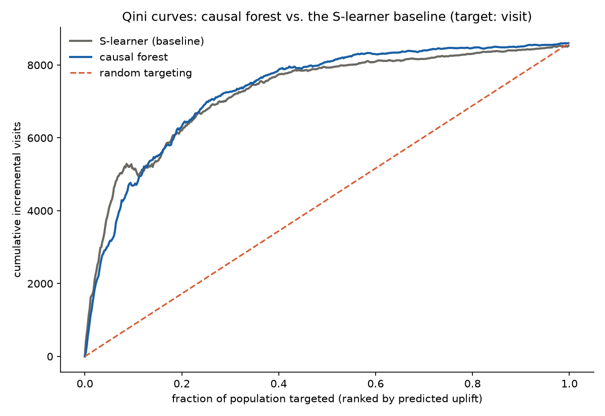
Both curves sit well above random targeting — real signal either way. The causal forest's edge over the baseline is visible but modest, matching the +1.8% number, not a dramatic separation.
This is the one method that beats the baseline, on both outcomes: +1.8% on visit, +3.8% on conversion. Modest, but real and consistent in direction rather than winning one outcome and losing the other by chance. The honest tradeoff is runtime: 518s and 713s per outcome against 4-10s for the meta-learners combined. Whether that's worth a low-single-digit Qini improvement is a real production question, not a rhetorical one. In a system retraining hourly it likely isn't. In a monthly targeting decision against a large ad budget, it easily could be.
What this is and isn't
S/T/X meta-learners are Kunzel et al. 2019's framework. Causal forests are Athey and Wager 2019's method. Nothing architecturally new in either. What's mine is implementing the meta-learners directly rather than calling a pre-built uplift library, and taking the validation problem seriously: checking methods against known ground truth before trusting them where none exists, and verifying the evaluation metric itself before relying on it as the only judge.
The finding isn't "sophisticated methods win" or "simple methods win." Both are true at once, depending on which question is being asked. If the question is whether a fast, simple approach captures the real signal, the S-learner already does, and the meta-learner machinery doesn't add anything here. If the question is what's the best achievable targeting, causal forest earns its extra cost with a real edge on both outcomes tested. Reporting only one half would be the misleading version of an otherwise complete result.
Code and every number above: github.com/Bauxitiego/uplift-modeling. Trained S-learner and causal forest models: huggingface.co/Bauxitiego/uplift-modeling — T-learner and X-learner aren't published as models, since they lost to the baseline on both targets tested. The Gate 0 synthetic benchmark, the one dataset here that's actually mine to publish: huggingface.co/datasets/Bauxitiego/uplift-modeling-synthetic-benchmark, 100,000 rows with a known, closed-form ground-truth treatment effect included.